ASTxplainer

Explaining Large Language Models for Code Using Syntax Structures

Abstract

Large Language Models (LLMs) for code are a family of high-parameter, transformer-based neural networks pre-trained on massive datasets of both natural and programming languages. These models are rapidly being employed in commercial AI-based developer tools, such as GitHub CoPilot. However, measuring and explaining their effectiveness on programming tasks is a challenging proposition, given their size and complexity. We believe that the methods for evaluating and explaining LLMs for code are inextricably linked. That is, in order to explain a model’s predictions, they must be reliably mapped to fine-grained, understandable concepts that helps developers to detect how good syntactic elements are being predicted by LLMs. Once this mapping is achieved, new methods for detailed model evaluations are possible. However, most current explainability techniques and evaluation benchmarks focus on model robustness or individual task performance, as opposed to interpreting model predictions.

To this end, this blog introduces ASTxplainer, an explainability method specific to LLMs for code that enables both new methods for LLM evaluation and AST visualizations of LLM predictions that aid end-users in understanding model predictions. At its core, ASTxplainer provides an automated method for aligning code token predictions with AST nodes, by extracting and aggregating normalized model logits within AST structures.

To demonstrate the practical benefit of ASTxplainer, we illustrate the insights that our framework can provide by performing an empirical evaluation on 12 popular LLMs for code using a curated dataset of the most popular GitHub projects. Additionally, we perform a user study examining the usefulness of an ASTxplainer-derived visualization of model predictions aimed at enabling model users to explain predictions. The results of these studies illustrate the potential for ASTxplainer to provide insights into LLM effectiveness, and aid end-users in understanding predictions (see our ArXiv paper).

Introduction

The advent and proliferation of online open-source code repositories and rapid advancements in transformer-based neural large language models LLMs have served as a catalyst for the advancement of automated Software Engineering (SE) tools with effectiveness. LLMs for code have demonstrated considerable proficiency across a diverse array of generative SE tasks, inclusive of, but not restricted to, code completion , program repair <d-cite key=Chen2019sequencer,ahmadunified2021></d-cite>, and test case generation . Moreover, these advancements are rapidly being introduced into commercial developer tools such as GitHub CoPilot and Replit’s Ghostwriter .

However, the sheer complexity and size that enable the often surprising effectiveness of LLMs for code is a double-edged sword. That is, while these attributes enable LLMs to capture important patterns in code that allow them to be applied to a range of programming tasks, effectively explaining and evaluating the capabilities of these models is a challenging proposition — they effectively function as black boxes that derive predictions from exceedingly complex internal model mechanics. Current research in both designing LLMs for code and in applying them to programming tasks typically makes use of existing benchmarks (e.g., CodeSearchNet~<d-cite key=husain2019codesearchnet}></d-cite>, or HumanEval~<d-cite key=chen_evaluating_2021}></d-cite> and metrics that have been adapted from the field of natural language processing (NLP) such as accuracy, BLEU, METEOR, and ROUGE, as well as more recent metrics further tailored for code such as CodeBLEU~. However, recent work has illustrated the limitations of benchmarks such as HumanEval~, and there has been growing criticism of automated metrics within the NLP community~<d-cite key=molnar2019interpret,Kim2018InterpretabilityTCAV,wan_what_2022,liu_reliability_2023></d-cite>. These deficiencies largely stem from the fact that such benchmarks and metrics are often targeted at evaluating functional or syntactic correctness of generated code or task performance, but are not able to explain model predictions or capabilities in an interpretable manner.

Methods for evaluating (i.e., the what) and explaining (i.e., the why) LLMs for code are inextricably linked to one another. An informative evaluation requires some degree of explainability of model predictions, such that model behavior can be understood at a fine-grained level. However, the fundamental challenge in achieving explainability of LLMs for code lies in establishing a reliable mapping mechanism that can bridge the gap between a given model’s predictions and human-understandable programming language (PL) concepts, which can aid in explaining the model’s decisions. As such, designing both effective evaluations and interpretability techniques for LLMs of code requires that one first establish this conceptual mapping.

Figure 1. Our proposed evaluative and explainability method is composed of ASC-EVal, ASC-Causal, and ASC-Viz.

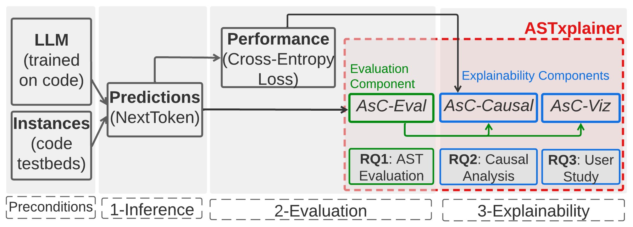
To overcome the challenges in explaining and evaluating LLMs for code, we propose a novel method for enabling a reliable conceptual mapping of LLMs predictions (i.e., the what) to PL concepts (i.e, the why), called ASTxplainer, which collects and aggregates LLMs token predictions into a construct that we call Abstract Syntax Concepts (ASC), derived from Abstract Syntax Trees (ASTs). By explicitly mapping model predictions to code structure, ASTxplainer provides a fine-grained methodology for examining how models perform relative to programming language concepts, and can help model end-users reason about why an LLMs may have made a certain set of predictions. ASTxplainer’s mapping of model predictions to ASC enables two new types of evaluations for LLMs of code, and one novel interpretability technique that visualizes model ASC to aid end users (i.e., developers using LLMs to auto-complete code) in understanding LLMs predictions. Fig.~1 illustrates these three main components of ASTxplainer.

The first evaluation technique, called ASCeval, is able to estimate the structural performance of a predicted syntax element in order to measure the uncertainty of the downstream code generative process (e.g., for code completion). The second evaluation technique called ASCcausal, is capable of generating causal explanations that link these structural performance values with canonical model performance (i.e., Cross-Entropy Loss). Finally, ASCviz implements a practical interpretability technique by visualizing model LLMs prediction uncertainty, organized into AST structures, aiding end-users in understanding the reliability of model predictions in practice. This blog concentrates on explaining ASCeval. The other techniques can be found on the preprint. We validate ASCeval and ASCcausal through a large-scale, comprehensive empirical study that evaluates 12 popular LLMs on a novel dataset of \(\approx\) 10 million tokens that are exclusive of the model’s training data. Furthermore, to evaluate the effectiveness of ASCviz, we conduct a user study examining the utility of multiple visualizations in aiding developers to understand and explaining model predictions. The results of our empirical study lead to novel insights regarding the performance of LLMs for code, and user study illustrates the promising utility of ASCviz.

Background & Related Work

ASTxplainer is an approach that converges the expectation of an evaluative technique with the rigurosity of an explainability technique to quantify the prediction uncertainty of LLMs for code. LLMs are the result of scaling up billions of parameters for context-aware word representations from pre-trained models . This section defines and formalizes the basic elements of our approach. We provide a definition of LLMs and how to evaluate them, the definition of Abstract Syntax Trees (ASTs) and how they were employed for probing, and finally, the explainability methods for LLMs.

Our research focused on LLMs because of their outstanding performance on code-based generative tasks. While other representations exist, such as graph-based models <d-cite key=allamanis2018learning,Allamanis19></d-cite>, we focus our discussion on sequence-based representations for simplicity. The goal of sequence-based models is to statistically learn a representation of a software artifact (e.g., snippet, comments, or test cases). We refer to SE-specific sequence-based data as a software corpus \(\mathcal{S}\). Given the sequential nature of \(\mathcal{S}\), we can decompose \(\mathcal{S}\) into a desired granularity of tokens, words, or sub-words by using a transformation function \(\Gamma(\mathcal{S})= w_1,...,w_I\) (i.e., tokenizers). This transformation function is a tokenization method for converting a software corpus into a sequence of discrete objects $w_i$ for \(1 \leqslant i \leqslant I\). Note that \(w_i \in V\), where the vocabulary \(V\) is a finite set.

Given this definition, a statistical language model is a probability distribution \(P\) over a fixed granularity of sequences of software corpora \(\mathcal{S}\). We can factorize the joint distribution over the \(i-\)dimension as:

\(P(\mathcal{S}) = P(w_1,...,w_I) = \prod_{i = 1}^{I} P(w_i | w_{<i})\).

Due to the discrete nature of the data, the expression \(P(w_i | w_{<i})\) can be estimated using a machine learning classifier. The classifier, in our particular case, is a Large Language Model (LLM) . Hence, rather than using n-grams or Markov Models to approximate \(P(w_i | w_{<i})\) , it is convenient to use a latent model \(P(w_i | w_{<i} ) \approx P(w_i | h_i )\), where \(h_i\) is known as a hidden state that embeds the sequence information from past observations up to the time step \(i\).

Depending on how the sequence is processed, the hidden state \(h_i\) can be computed using either Encoder-Only, Encoder-Decoder, or Decoder-Only architectures according to the transformers’ layers One popular bidirectional objective function used widely in representation learning is masked language modeling . This function aims to predict masked text pieces based on the surrounding context. CodeBERT , CuBERT (345M) CodeRoBERTa , and GraphCodeBERT are examples of Encoder-Only models for code. In programming contexts, these methods provide useful representations of code sequences for downstream tasks such as code classification, clone and defect detection. CodeT5 and PLBART are examples of Encoder-Decoder models. These models encode an input sequence and, then, this encoded sequence is decoded with a different architecture. Encoder-Decoder models are trained with the goal of reconstructing masked input sequences . Additionally, they have been employed for SE tasks such as code summarization, and code generation using masks. Finally, Decoder-Only models predict the probability of a token given a preceding sequence. CodeGPT , CodeParrot , GPT-Neo , GPT-J , Codex , GPT-NeoX , and Google's left-to-right decoder-only Transformer language models <d-cite key=vaswani2017transformers,austin2021program> are examples of _Decoder-Only_ models for code.

Although our proposed approach ASTxplainer was designed to be compatible with either type of LLMs, this research concentrated on Decoder-Only models due to their popularity for code-based generative tasks . Decoder-based models share a common property: the ability to connect previously processed information to a present task, such as using an initial sequence of tokens to predict new code tokens. The resulting auto-completed sequence should be coherent with respect to the context of the initial sequence. This property is known as the ability to model long-range dependencies .

Definition 1. [Decoder-Only Transformers]: Decoder-Only models update the hidden state \(h_i = f(h_{i-1}, w_{<i})\) using past inputs \(w_{<i}\) and a previous hidden state \(h_{i-1}\). In other words, these models function in a feed-forward manner that predicts future values from historical values directly. LLMs trained on source code have the ability to generate tokens or sub-words given a history. Hence, decoder-only models are employed as generative models:

\(\hat{w_i} \approx P(w_i | w_{<i} ) = \sigma(y)_i = \frac{e^{y_{w_i}}}{\Sigma_j e^{y_j}}\).

In the previous approximation, the predicted token \(w_i\) is conditioned by the past information. The term \(y_j\) represents the non-normalized log-probabilities for each output token \(j\). We extracted and normalized these log-probabilities from the last layer of LLMs to estimate the Next-token Predictions (NtP) in ASTxplainer . This estimation relies on the softmax function. The softmax \(\sigma_i\) returns a distribution over predicted output classes, in this case, the classes are each token in the previously introduced vocabulary \(V\). It is expected that the predictions contained in \(\sigma_i\) are influenced by previous inputs of the sequence \(w_{<i}\).

Probing is a supervised analysis to determine which type of parameters (e.g., input code snippets, tokenization process, number of hidden layers, and model size) influence the learning process in machine learning models . The purpose of probing is to assess whether hidden representations of machine learning models (i.e., LLMs) encode specific linguistic properties such as syntactic structures of programming languages. For example, Lopez et al., trained a linear classifier to show that code syntactic structures are encoded in pre-trained models in the form of Abstract Syntax Trees (ASTs). Lopez et al.’s approach demonstrates that the middle layers of pre-trained models contain ASTs’ information.

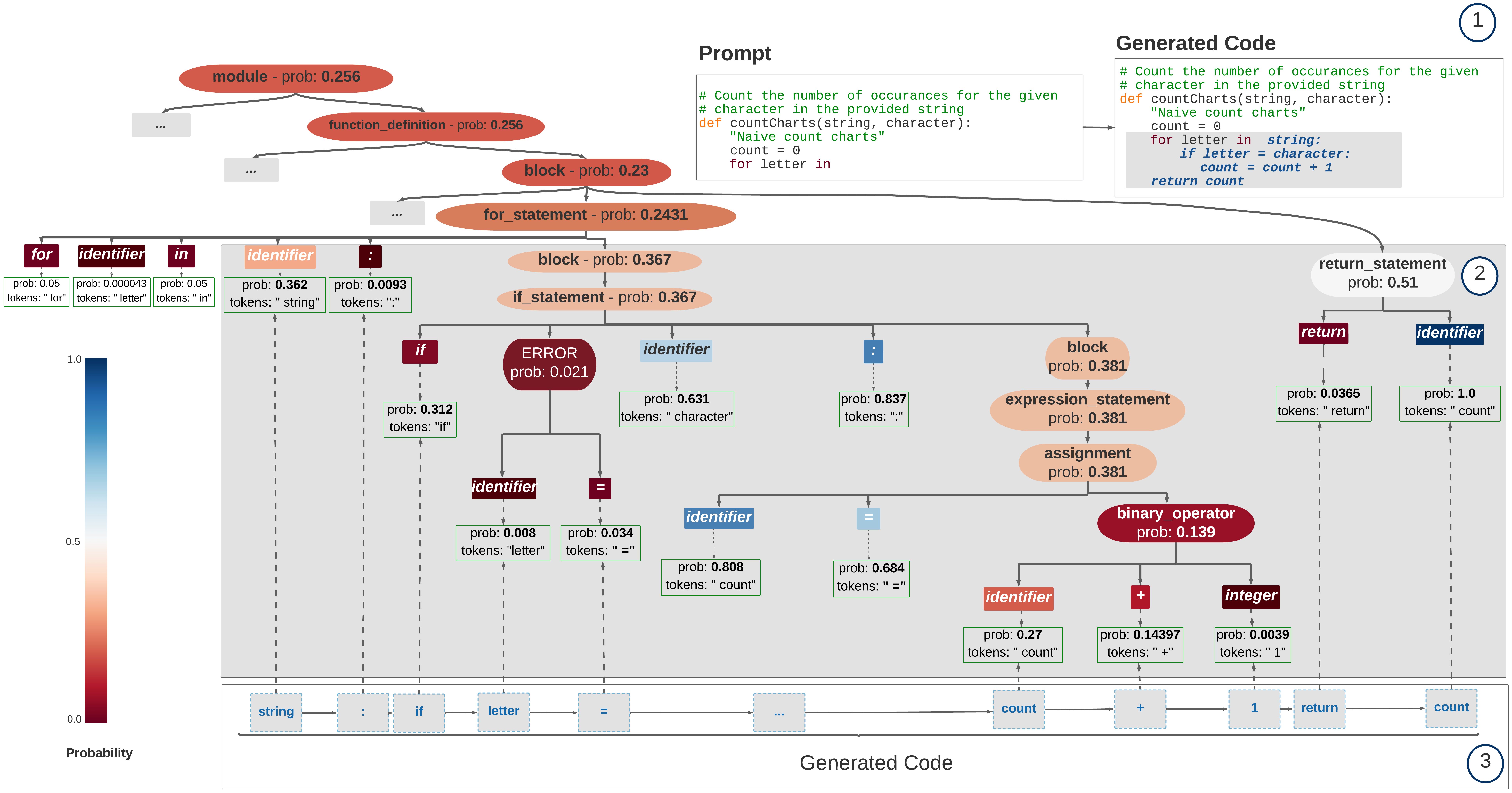
Nonetheless, instead of proposing another syntax probe, our approach ASTxplainer adapts AST information to evaluate and explain LLMs. ASTs are defined as a formal representation of syntactical structures built upon linguistic elements of PLs. ASTs are formed according to the production rules defined in Context Free Grammar (CFGs). More precisely, production rules are functions that combine terminal and non-terminal nodes into statements. Terminal nodes are symbols in the source code (e.g., tokens in region (3) of Fig.~2), while non-terminal nodes encapsulate more than one terminal node to define the structure of a statement (e.g., nodes containing children in region (2) of Fig.~2).

When designing our approach ASTxplainer , we leveraged meaningful and interpretable information defined in Context-Free Grammars (\(CFGs\)). \(CFGs\) are a set of rules containing the syntax and structural information of a language <d-cite key=10.5555/1196416></d-cite>. Ultimately CFGs define instructions that specify how different tokens (i.e., Lexemes) are put together to form valid statements in every programming language.

Definition 2. [Context Free Grammars]: $CFG$ \(\mathbb{G}\) is expressed as \(\mathbb{G} = (\alpha, \lambda, \omega, \beta)\) where \(\alpha\) denotes the finite set of non-terminal symbols, \(\lambda\) the finite set of terminal symbols, \(\omega\) the finite set of production rules and \(\beta\) the start symbol. The set of production rules \(\omega\) for any type of statement (e.g., conditional, assignation, operator) is expressed in terms of the terminal and non-terminal symbols.

Figure 2. Local Evaluation for code Completion.

The ASC-Eval Component

LLMs for code can be considered a black box because of their uncertain behavior when predicting tokens. To estimate such uncertainty, we can employ explainability methods on LLMs. Explainability aims to understand how a model operates and comes to decisions either by exploring inner layers or performing perturbation analysis on the models’ inputs <d-cite key=belleprinciples2020,molnarinterpretable2020></d-cite>. For example, Gholizadeh et al., propose a local explainability technique, namely layer-wise relevant propagation (LRP), that computes the importance of an interpretable n-gram in classifying a text sequence. LRP calculates a score with the sum of activated weights during the back-propagation to identify the most influential n-grams. This score is employed for explaining the importance of a given n-gram for a canonical (i.e., SVM) and a neural model(i.e., CNN). The authors demonstrated that LRP outperforms the gradient-only-based and permutation-only-based explainability techniques . It is important to clarify that, in our research, explainability and interpretability are used interchangeably. However, the goal of our research is to introduce a technique that provide a fine-grained explanation of accuracy-based metrics based on syntax elements of Programming Languages.

In the context of pre-trained models for code, Liu et al., experimented with Encoder-Decoder models for code2code and comment2code tasks (e.g., T5, CodeText, and CodeTrans). Their research aims at explaining why neural models generate code sequences reliably by identifying tokens that contribute the most to a sequence prediction . Moreover, Vasconcelos et al., propose a technique that highlights generated code using an uncertainty threshold. Their approach points out fragments of the sequence where developers can intervene upon the uncertainty threshold . On the other hand, we can explain pre-trained models for code using structural information. For instance, Wan et al., conducted an interpretability analysis on Encoder-only models (e.g., CodeBert and GraphCodeBert) focusing on three aspects: 1) how the self-attention weights align with the syntax structure, 2) whether the syntax structure is encoded in the hidden layers, and 3) how pre-trained models induce syntax structure .

Even though previous research has introduced explainability techniques to analyze pre-trained models with structural information, those techniques have been tested and designed for modest-size Encoder-Only models (i.e., less than 1B). Conversely, our study ASTxplainer proposes not only an explainability technique that contextualizes canonical metrics (i.e., cross-entropy loss) based on causal inference but also an evaluative metric (ASCeval) for Decoder-only LLMs that predicts ASTs terminal and non-terminal nodes. More importantly, we introduce and control a set of confounders based on code features (e.g., AST-levels, AST-nodes, and number of tokens) to properly estimate the relationship between ASCeval and canonical metrics (see Tab.~2 in our preprint).

Kim et al., introduce a formal mathematical structure known as a function for explainability (\(\varphi\)). We use this definition to formally describe what constitutes an explainable method in SE. Most LLMs for code operate by predicting tokens \(P(w_i | d_i)\) that do not inherently match high-level concepts a human can easily understand. Kim et al., claim that such difficulty can be expressed mathematically as representing the state of LLMs as a vector space (\(\vec{m}\)). Conversely, humans or, in our study, developers operate in a different vector space \(\vec{h}\), which corresponds to an unknown set of human-interpretable concepts (\(h\)). As such, our main challenge is to map \(\vec{m} \to \vec{h}\) bridging this gap between the disparate vector spaces. The key insight of ASTxplainer is the formalization of an explainability function \(\varphi\) for LLMs of code.

Definition 3. [Interpretability Function for Next Token Predictions]: Consider \(\varphi: \vec{m} \to \vec{h}\). In this formulation, \(\vec{m}\) represents an approximation of a model’s vector space as measured through token prediction performance at different granularity levels (i.e., normalized log-probabilities). This vector space approximation is then mapped to human-understandable concepts \(\vec{h}\) that represent programming language syntactic concepts (i.e., terminal and non-terminal nodes).

While LLMs have seen striking advances with regard to code generation and other downstream SE tasks <d-cite key=Chen2021EvaluatingCode,watson2020dl4se></d-cite>, researchers are still not able to evaluate what aspects of code are actually statistically learned by these models. In this section, we propose a new metric, ASCeval, to showcase the statistical behavior of syntactic elements generated by LLMs. Our proposed ASCeval comprises the basic units for explainability as Abstract Syntax Concepts (ASC), an alignment function \(\delta\) that links tokens with ASTs, and an aggregation function \(\theta\) that estimates the prediction performance of a terminal and non-terminal nodes. We propose an explainability function \(\varphi\) that relies on the alignment function $\delta$ and the aggregation function \(\theta\) to perform the mapping from log-probabilites (i.e., NtP) to developer-understandable concepts (i.e., ASC).

Figure 3. _ASC_eval Components. Left: Nodes are employed as ``concepts''. Center: Each token is aligned to the end nodes of the AST with an offset function. Right: Node probabilities are estimated with an aggregation function.

Abstract Syntax Concepts ($ASC$)

ASCeval can be formally defined (see Def.~3) as an explainability function \(\varphi\) of token predictions of LLMs using Context Free Grammars. We introduce the term Abstract Syntax Concepts (ASC) to represent the terminal and non-terminal symbols in a Context Free Grammar (see Def~.2). Specifically, to approximate a LLMs’ vector space, in \(\vec{m}\), we extract the last layer to calculate NtP, which is, in fact, a generative measure of performance. Then in \(\vec{h}\), we map the model’s prediction performance at the token level (NtP) to ASC (for which we define a set of categories $\mathcal{H}$), to make it easier to interpret what aspects of LLMs are effective or erroneous at predicting.

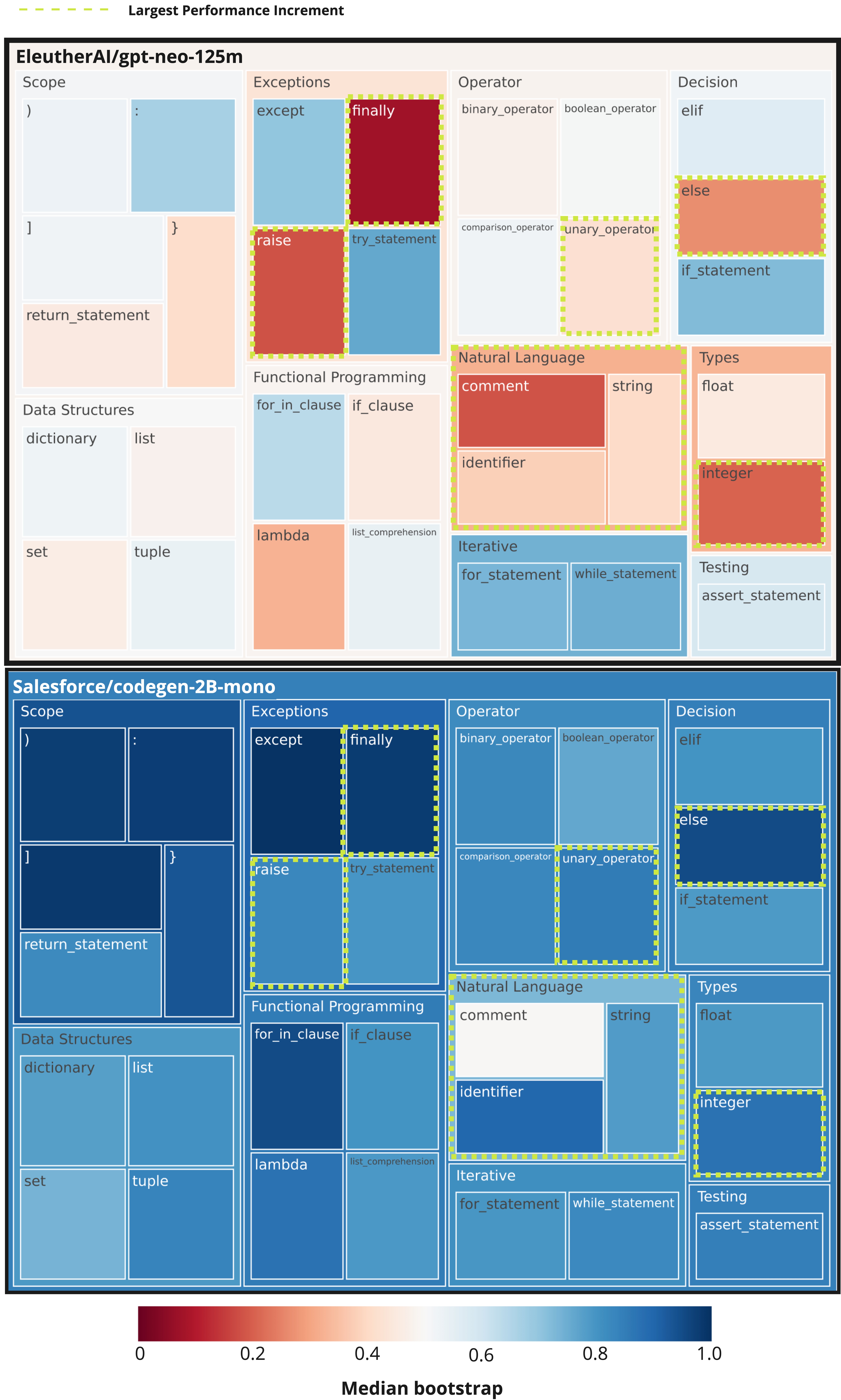
In PLs, terminal and non-terminal nodes retain different semantic meanings. For instance, identifier and string nodes correspond to a common Natural Language concept category. As such, we can group nodes $n$ into semantically meaningful categories \(\mathcal{H}\). Fig.~\ref{fig:largeTreeMap} depicts some of our proposed categories for Python. These categories will allow ASCeval to assign semantic meaning to predicted ASC. ASC are the fundamental mathematical units for enabling the evaluation and explainability of LLMs. Fig.~4 depicts some of the concepts used to evaluate LLMs with ASCeval. Concepts \(n \in N\) are types of symbols defined by tree-sitter’s $CFG$ <d-cite key=tree-sitter></d-cite>. In summary, Each token in a sequence \(s\) can be assigned to a category \(h \in \mathcal{H}\). With our categories \(\mathcal{H}\), researchers and developers can easily associate LLMs’ performance to particular structural code attributes. As such, ASCeval allows for LLMs Next-token Predictions to be explained in a developer-centric way.

Fig~3-A depicts the AST representation of a Python snippet of a naive implementation of the function \(countCharts\). This function counts and returns the number of occurrences of a given character for an input string. In the AST representation, the leaf nodes correspond to the terminal tokens used in the snippet, while the intermediate nodes correspond to non-terminals. Our approach relies on the tree-sitter library <d-cite key=tree-sitter></d-cite> to construct the AST representations of the snippets. Once the AST has been parsed, we can access the information for all nodes and retrieve useful properties such as their type, children, and location.

AST Alignment function ($\delta$)

Figure~3-B illustrates the process of aligning terminal and non-terminal nodes in the AST representation with their corresponding tokens. Prior to this alignment process, we split the $countCharts$ snippet \(s\) into tokens using the model tokenizer \(\Gamma(s) = (w_1,...,w_i)\). Since the tokenizer may produce a sequence of tokens where each token does not necessarily matches with a single terminal node, a single node in the AST may contain more than one associated token. In fact, intermediate nodes are aligned with a sub-sequence of the original snippet rather than a single token. We define for this purpose the alignment function \(\delta: N \to s_{<=i}\) where \(s_{<=i}\) corresponds to a subsequence of a snippet and $N$ is the set of terminal and non-terminal nodes. We leverage the offset property of each AST node to conduct this process, in other words, we search for all the tokens in \(s\) that are located within the offset range of each node. To illustrate how function $\delta$ works, let’s consider the example in Figure~3-B, in the sub-tree the terminal node ( is aligned with token {(} while the sibling node identifier is aligned with tokens {str} {ing}. The parent node parameters will be consequently aligned with {(} {str} {ing} {,} {char} {acter} {)}.

AST Aggregation function (\(\theta\))

We design an aggregation function \(\theta\) that computes our proposed metric ASCeval, which represents how confident a terminal or non-terminal node $n$ is predicted by an \llm. By relating these node predictions to an actual node symbol, we gain an understanding of how well a studied model is generating code. These ASCeval performance values can also uncover specific long-range interactions and map them into an AST visual structure (see Sec.~\ref{sec:approach-3}). ASCeval performs at two levels of granularity depending on the scope of the analyzed corpus \(\mathcal{S}\). We refer to such granularity as local and global aggregation. Local aggregations operate for a code snippet, while global aggregations operate for a corpus. Although local aggregation can provide a ASCeval value for a single snippet, this aggregation allows computing an average of aggregated values at snippet granularity.

Figure~3-C shows the aggregation function used to compute the prediction probability for each node. Once the tokens are aligned with their corresponding nodes using \(\delta\), we traverse the entire AST and aggregate the NtP probabilities of their associated tokens. The aggregation function \(\theta\) can take the form of a statistical average, median or max values depending on the user configuration. In our study, we set the aggregation \(\theta: N \to median(\delta(N))\) for a subset of tokens \(s_{<=i}\). For example, as illustrated in Fig.~3-C, the parent node parameters has an associated average value of $0.23$. This parent node average was aggregated with its terminal values: ( with \(0.07\), identifier with $0.4$, , with \(0.5\), identifier with $0.1$, and ) with $0.1$.

Figure 4. `ASCeval` for 10 _ASC_ Categories and 2 LLMs (\monoIIII and \gptI).

Results

In order to illustrate the insights that ASTxplainer can enable, we present an empirical evaluation on 12 LLMs, which shows how LLMs behave for each Abstract Syntax Concept, and a user study, which assesses the usability of our approach. This section details the methodological steps and results for only the first research question. Please refer to the pre-print for the other questions and further details.

$RQ_1$: To what extent do Large Language Models for code predict syntactic structures?

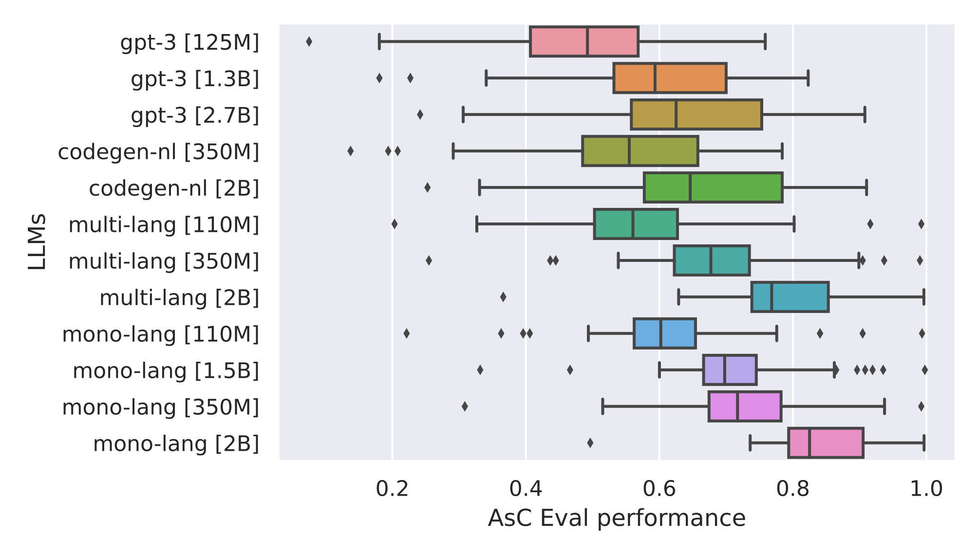
To answer $RQ_1$, we generated the normalized log-probabilities or Next Token Predictions (NtP) for each code snippet in $\mathcal{S}=$ galeras. These log-probabilities were extracted at inference time for each token position for the 12 LLMs. The log-probabilities distributions have a vector size of |\(V\)| for each token position in \(s \in \mathcal{S}\). These distributions are processed to obtain the log-probability that actually matches the expected token in a position \(i\). Therefore, each token position has an associated prediction value that we save for generating the NtP sequence. Such Next-token Prediction sequence is the input for the aggregation function \(\theta\) that generates the corresponding ASCeval values. Additionally, we computed the cross-entropy loss of each snippet \(s\) in our dataset. To obtain the ASCeval Global value in Tab.~1 and Fig.~5, we aggregated ASCeval performance values (i.e., all available $ASC$) by LLM. The values per model are bootstrapped with the median (size of 500 samplings) to enable a fair comparison among models. Similarly, to obtain the ASCeval per Abstract Syntax Concept Category (e.g., Data Str, Decision, or Scope), we globally aggregated performance values of tokens under these categories. We also explored with Type Model aggregations.

Table 1. Large Language Models characteristics and their associated `ASCeval` performance. Erroneous `ASCeval` values are in red. Confident `ASCeval` values are in blue. Best global `ASCeval` is underlined.

In this $RQ_1$, we provide an empirical value (bootstrapped median columns in Tab.~1) of the prediction of Abstract Syntax Concepts for the 12 LLMs. We set a threshold of $0.6$ as an acceptable rate of prediction confidence for our ASCeval metric. Fig.~4, for example, shows our best and worst LLMs, mono-lang [2B] and gpt-3 [125M] respectively, at every proposed Abstract Syntax Concept. We observe that, in general, scaling the parameters of LLMs plays a fundamental role in the prediction of $ASC$. The dashed green boxes show the largest ASCeval performance increments from the worst to the best concepts. Particularly, {Exceptions}, {Natural Language}, {Operators}, {Types}, and {Decisions} present the biggest jumps in syntactic ASCeval performance.

Our empirical evaluation shows that $ASC$ categories that fulfill the $0.6$ threshold for the 12 LLMs are {Scope} with the highest ASCeval performance of $0.94$ for the Mono-Language-Type models, {Iterations} with $0.82$ for codegen-nl [2B], and {Testing} with $0.85$ for mono-lang [2B] (see Tab.~1). Conversely, we found some concept categories struggle with ASCeval performance. We refer to these categories as {erroneous} since they are below $0.5$. Those categories are mainly {Natural Language} category with the largest average median of $0.46$ and {Data Types} with the largest average median of $0.47$ for NL GPT-3.

We believe that models poorly behave with low ASCeval performance because category concepts such as {Natural Language} and {Data Types} require more context to be accurately predicted. For instance, the string concept requires a larger window context before properly being predicted. Similarly, the category {Data Types} is prone to be erroneous since they may appear more frequently at the beginning of the snippets compared to other categories. Also, bear in mind that {Data Types} are less frequent concepts due to the dynamic typing for Python. In general, none of the evaluated architectures performed well at predicting {Data Types} accurately except by mono-lang [2B], which was trained with a large number of code samples.

Table~1 depicts that {Iteration} category mostly surpasses the threshold for all our models except for codeparrot-small-multi with an average median ASCeval of $0.6$. From our smaller models (i.e., in a range of millions of parameters), the lowest average median obtained for gpt-3 [125M] is $0.74$, which also surpasses the threshold. This outstanding behavior of NL GPT-3 models could be explained as Python reserved words for iterations such as for and while also appear in natural language with similar semantics.

Figure 5. `ASCeval` Performance grouped by specific LLMs and `ASCeval` density by Model Type.

Fig.~5 indicates that models trained on natural language have more median variability than models fine-tuned on code datasets. For instance, NL GPT-3 and NL Codegen report values in a range from $0.2$ to $0.9$. Conversely, fine-tuned models with code such as Mono-Language-Type has a lower variability than NL GPT-3 and NL Codegen categories. For example, mono-lang [2B] has a global avg. median ASCeval of $0.84$ and a variability range between $0.7$ and $1.0$, outperforming the $0.6$ threshold. Furthermore, mono-lang [2B] is our best model with an average global ASCeval of $0.84$. On one hand, this suggests that fine-tuned models on code are predicting $ASC$ with higher confidence than natural language-only models. On the other hand, although Multi-Language-Type models exhibit high variability (from $0.5$ to $0.9$), their average median ASCeval (i.e., $0.68$ for multi-lang [110M]) is even better than natural language models (i.e., $0.48$ with variability from $0.2$ to $0.8$ for gpt-3 [125M]).

Citation

@misc{palacio_evaluating_2023,
	title = {Evaluating and Explaining Large Language Models for Code Using Syntactic Structures},
	url = {http://arxiv.org/abs/2308.03873},
	publisher = ,
	author = {Palacio, David N. and Velasco, Alejandro and Rodriguez-Cardenas, Daniel and Moran, Kevin and Poshyvanyk, Denys},
	urldate = {2023-08-22},
	date = {2023-08-07},
	langid = {english},
	eprinttype = {arxiv},
	eprint = {2308.03873 [cs]},
}